Capabilities
TEXES will be used for echelle slit spectroscopy in the 5 to 25 micron wavelength region. TEXES has a resolution (λ/δλ where δλ is the FWHM of spectral lines, about 3 pixels) of 100,000 at wavelengths shorter than 10 microns, and a fixed wavenumber resolution of 0.01 inverse cm at longer wavelengths. Thus the resolution is between 100,000 and 40,000, the walue being inversely proportional to the wavelength, for wavelengths between 10 and 25 microns.
The wavelength coverage is from 5 to 20 microns and from 22 to 25 microns. The wavelengths from 20 to 22 microns are inaccessible for the echelle. Wavelengths from 5.5 to 8 microns and 14 to 16.9 microns are either mostly or comletely blocked by the atmosphere. However the molecular Hydrogen line at 17.05 microns can be observed with TEXES. Pls should consult detailed plots of the atmospheric transmission expected at Mauna Kea to see that the wavelength they wish to observe can actually be observed, given whatever atmospheric absorption lines are going to be present. While observations can be carried down to 5 microns, the TEXES detector has poor sensitivity at wavelengths near 5 microns compared to the InSb detectors used in most modern near-infrared instruments.
Observing Modes
| TEXES STANDARD OBSERVING CONFIGURATIONS RESOLVING POWERS, WAVELENGTH COVERAGES, SLIT LENGTHS |
| 5-14μm 0.52 arcsec wide slit |
17-20μ, 22-25μm 0.75 arcsec wide slit |
| R~85,000 (high) Δλ ~ 0.006 λ slit length: 4 arcsec |
R~60,000 (high) Δλ ~ 0.006 λ slit length: 8 arcsec |
| R~85,000 (high) Δλ ~ 0.25μm slit length: 1.7 arcsec |
- |
| R~15,000 (medium) Δλ ~ 0.006 λ slit length: 20 arcsec |
R~11,000 (medium) Δλ ~ 0.006 λ slit length: 20 arcsec |
| R~4,000 (low) Δλ ~ 0.25μm slit length: 20 arcsec (8-14μm only) |
- |
The usual operating procedure for TEXES is to nod the target along the slit during the observation, so that taking the difference of the observations at the two positions removes the sky emission. It is also possible to scan the slit across an extended target, such as a planet, to produce a spatial map of the spectrum. Pls should consult with the TEXES team concerning the suitability of these nodes for whatever observations they wish to carry out.
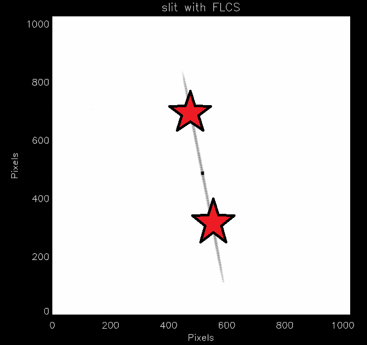
The object alternates between the two points |
[Source: Irons et al. 2012 ApJ 755 90] |
Sensitivity
To be consistent with the sensitivity tables for Michelle, values are given in terms of the source brightness for which S/N = 5 in 1 hour (total clock time). TEXES normally TEXES peaks up on the target during acquisition, and this would be difficult on a target that is so faint as to only get S/N of 5 in 1 hour. PIs should bear in mind the difficultly of acquiring very faint targets with TEXES. The only circumstances where acquisition would be easy for a faint target is either if the acquisition can be done on a nearby bright target, followed by an offset to put the faint target on the slit [see below], or if a target is optically bright in which case it should be possible to place it on the TEXES "hotspot" directly during the acquisition.
| Resolution mode | Resolution1 | Surface2 Brightness erg / (s cm sr cm-1) 5 σ 1 min | Line3 Brightness erg / (s cm sr) 5 σ 1 min | Point source4 flux density (mJy) 5 σ 1 hr |
Point source5 magnitude 5 σ 1 hr |
|||
| 10 μm | 20 μm | 8 μm | 12 μm | 20 μm | ||||
| low | 0.003μm | 6 x 10⁻³ | 3 x 10⁻³ | 30 | 60 | 8.5 | 7.2 | 5.5 |
| medium | 24 km/s | 1.5 x 10⁻² | 2 x 10⁻³ | 70 | 140 | 7.6 | 6.3 | 4.6 |
| high | 3.6 km/s | 6 x 10⁻² | 8 x 10⁻⁴ | 250 | 500 | 6.2 | 4.9 | 3.2 |
1 Low-res wavelength resolution and high-res velocity resolution are approximately constant with wavelength. Medium-res velocity resolution is roughly constant, but varies with wavelength within the grating orders.
2 Spectrally and spatially resolved surface brightness sensitivity is approximately constant with wavelength, assuming a transpararent atmosphere. Sensitivities are for 1 sigma 1 second per spatial resolution in a scan map, or 5 sigma in 1 minute of clock time per spatial resolution element, including time for overheads and sky measurements. For one position in a spatially extended source observed by nodding the telescope off of the source, 2 minutes of clock time are required for a 5 sigma detection.
3 Spatially resolved line brightness sensitivity for a narrow line is approximately constant with wavelength, assuming a transpararent atmosphere. Units are erg/(s cm2 sr) or 1x10⁻³ W/(m2 sr). Numbers are for 1 sigma in 1 second spent per spatial resolution element in a scan map, or 5 sigma in 1 minute clock time per spatial resolution element, including time for overheads and sky measurements.
4 Spectrally resolved point-source flux sensitivity varies approximately linearly with wavelength, assuming a transparent atmosphere. Numbers are for 5 sigma in 1 hour of clock time for a point source nodded along the slit, and include light loss at the slit.
5 Point source magnitudes for 5 sigma detections in 1 hour of clock time, assuming a transparent atmosphere.
Effects of Atmosphere
Due to the significant variations in the sensitivity with wavelength, prospective PIs are encouraged to contact members of the TEXES team for help with the sensitivity estimates for their specific wavelengths of interest.
The above estimates are assuming that the target is in the slit at both nod positions. If it is necessary to nod the target off of the slit--which is likely to be the case for extended targets--then the on-target efficiency is 2 times poorer than assumed. For such cases the sensitivities will be 1.4 times worse than shown above.
The observations at 5-13 micron are assumed to be at wavelengths where the atmosphere is essentially transparent (< 3% atmospheric emissivity or 10% total with instrument and telescope) and those at 17-24 micron are assumed to be made with 20% total background emissivity. To determine the sensitivity at a specific wavelength, it is necessary to determine the atmospheric emissivity and multiply by
(1+atmo_emiss/.1)0.5/(.93-atmo_emiss) at 5-13 micron,
or
(1+atmo_emiss/.2)0.5/(.93-atmo_emiss) at 17-24 micron.
It is not uncommon for this factor to degrade the sensitivity by a factor of 2. In addition, the instrumental response rolls off between echelon orders, which can degrade the sensitivity by an additional factor of 1.4. The line sensitivities assume the line is narrow compared to the resolution of λ/100,000 shortward of 10 micron and 0.01 cm-1 longward. For broader lines, the sensitivity numbers must be multiplied by the square root of the number of resolution elements over which the line is spread, or the NEFD numbers could be used.